PLOTTING RESULTS ON XGRAPH or GNUPLOT

XGraph

The xgraph program draws a graph on an X display given data read from either data files or from standard input if no files are specified. It can display up to 64 independent data sets using different colors and/or line styles for each set. It annotates the graph with a title, axis labels, grid lines or tick marks, grid labels, and a legend. There are options to control the appearance of most components of the graph.

A data set consists of an ordered list of points of the form “directive X Y”. For directive “draw”, a line will be drawn between the previous point and the current point. Specifying a “move” directive tells xgraph not to draw a line between the points. “draw” is the default directive. The name of a data set can be specified by enclosing the name in double quotes.

The interface used to specify the size and location of this window depends on the window manager currently in use. Once the window has been opened, all of the data sets will be displayed graphically with a legend in the upper right corner of the screen.

Xgraph also presents three control buttons in the upper left corner of each window: Hardcopy, Close and about xgraph accepts a large number of options most of which can be specified either on the command line, in the user’s .Xdefaults or .Xresources file, or in the data files themselves.

The xgraph can be installed to your linux by using the below code on the terminal window;

In Ubuntu 10.10 you can now install ns,nam and xgraph by just a single command in the Terminal:

$ sudo apt-get install ns2 nam xgraph

You will be prompted for the user password. Enter it and watch Ubuntu 10.10 do the things for You!

The following program shows how XGraph can be used to plot the bandwidth of two nodes connected through full duplex wired link.

#Create a simulator object

set ns [new Simulator]
#Open the output trace file
set f0 [open out0.tr w]
#Create 2 nodes
set n0 [$ns node]
set n1 [$ns node]
#Connect the nodes using duplex link
$ns duplex-link $n0 $n1 1Mb 100ms DropTail
#Define a 'finish' procedure
proc finish {} {
        global f0
        #Close the output files
        close $f0
        #Call xgraph to display the results
        exec xgraph out0.tr -geometry 800x400 &
        exit 0
}
#Define a procedure which periodically records the bandwidth received by the
#the traffic sink0 and writes it to the file f0.
proc record {} {
        global sink0 f0
    #Get an instance of the simulator
    set ns [Simulator instance]
    #Set the time after which the procedure should be called again
        set time 0.5
    #How many bytes have been received by the traffic sinks?
        set bw0 [$sink0 set bytes_]
    #Get the current time
        set now [$ns now]
    #Calculate the bandwidth (in MBit/s) and write it to the files
        puts $f0 "$now [expr $bw0/$time*8/1000000]"
    #Reset the bytes_ values on the traffic sinks
        $sink0 set bytes_ 0
    #Re-schedule the procedure
        $ns at [expr $now+$time] "record"
}
#Create three traffic sinks and attach them to the node n4
set sink0 [new Agent/LossMonitor]
#Start logging the received bandwidth

$ns at 0.0 "record"
$ns at 60.0 "finish"
#Run the simulation
$ns run

xgraph plot of  the above program

 ====================================================================

More improvements on XGraph

In the above program we can see that the xgraph is called and and the output is plotted by using the finish procedure; 

ie:

    #Define a 'finish' procedure

    proc finish {} {

        global f0

        #Close the output files

        close $f0

        #Call xgraph to display the results

        exec xgraph out0.tr -geometry 800x400 &

        exit 0

   }

  

The following commands can be used to improve the appearance of xgraph . Add these commands on the end of "exec xgraph out0.tr -geometry 800x400 &" line in the above finish procedure;and observe the change.

1) -geometry WxH+X+Y or /=WxH+X+Y (Geometry)

Specifies the initial size and location of the xgraph window.

2) -bar (BarGraph)

Specifies that vertical bars should be drawn from the data points to a base point which can be specified with -brb. Usually, the -nl flag is used with this option. The point itself is located at the center of the bar.

3) -fitx

Translate and scale the x data from all datasets to fit [0. . . 1].

4) -fity

Translate and scale the y data from all datasets to fit [0. . . 1].

5) -fmtx <printf-format> -fmty <printf-format>

Use the format specified to generate the legends for the x or y axis.

6) -bb (BoundBox)

Draw a bounding box around the data region. This is very useful if you

prefer to see tick marks rather than grid lines (see -tk).

7) -bd <color> (Border)

This specifies the border color of the xgraph window.

8) -bg <color> (Background)

Background color of the xgraph window.

9) -brb <base> (BarBase)

This specifies the base for a bar graph. By default, the base is zero.

10) -brw <width> (BarWidth)

This specifies the width of bars in a bar graph. The amount is specified

in the user’s units. By default, a bar one pixel wide is drawn.

11) -bw <size> (BorderSize)

Border width (in pixels) of the xgraph window.

12) -fg <color> (Foreground)

Foreground color. This color is used to draw all text and the normal grid lines in the window.

13) -gw (GridSize)

Width, in pixels, of normal grid lines.

14) -gs (GridStyle)

Line style pattern of normal grid lines.

15) -lf <fontname> (LabelFont)

Label font. All axis labels and grid labels are drawn using this font. A font name may be specified exactly (e.g. ”9x15” or ”-*-courier-bold-rnormal-*-140-*”) or in an abbreviated form: ¡family¿-¡size¿. The family is the family name (like helvetica) and the size is the font size in points (like 12). The default for this parameter is ”helvetica-12”.

16) -lnx (LogX)

Specifies a logarithmic X axis. Grid labels represent powers of ten.

17) -lny (LogY)

Specifies a logarithmic Y axis. Grid labels represent powers of ten.

18) -lw width (LineWidth)

Specifies the width of the data lines in pixels. The default is zero.

19) -lx <xl,xh> (XLowLimit, XHighLimit)

This option limits the range of the X axis to the specified interval. This (along with -ly) can be used to ”zoom in” on a particularly interesting portion of a larger graph.

20) -ly <yl,yh> (YLowLimit, YHighLimit)

This option limits the range of the Y axis to the specified interval.

21) -m (Markers)

Mark each data point with a distinctive marker. There are eight distinctive markers used by xgraph. These markers are assigned uniquely to each different line style on black and white machines and varies with each color on color machines.

22) -M (StyleMarkers)

Similar to -m but markers are assigned uniquely to each eight consecutive data sets (this corresponds to each different line style on color machines).

23) -nl (NoLines)

Turn off drawing lines. When used with -m, -M, -p, or -P this can be used to produce scatter plots. When used with -bar, it can be used to produce standard bar graphs.

24) ng (NoLegend)

Turn off drawing Legends. Can be used to increase the drawing area.

25) -t <string> (TitleText)

Title of the plot. This string is centered at the top of the graph.

26) -tf <fontname> (TitleFont)

Title font. This is the name of the font to use for the graph title. A font name may be specified exactly (e.g. ”9x15” or ”-*-courier-bold-r-normal-*-140-*”) or in an abbreviated form: ¡family¿-¡size¿. The family is the family name (like helvetica) and the size is the font size in points (like 12). The default for this parameter is ”helvetica-18”.

27) -x <unitname> (XUnitText)

This is the unit name for the X axis. Its default is ”X”.

30) -y <unitname> (YUnitText)

This is the unit name for the Y axis. Its default is ”Y”.

31) -zg <color> (ZeroColor)

This is the color used to draw the zero grid line.

32) -zw <width> (ZeroWidth)

This is the width of the zero grid line in pixels.

example:

    #Define a 'finish' procedure

    proc finish {} {

        global f0

        #Close the output files

        close $f0

        #Call xgraph to display the results

        exec xgraph out0.tr -geometry 800x400 & -bar -fitx -fity -bb -bg white

        exit 0

   }

you can download an example program for plotting xgraph from here

Gnu PLOT

 

1. INSTALLING AND STARTING GNUPLOT 

Gnuplot is a free, command-driven, interactive, function and data plotting program. Pre-compiled executeables and source code for Gnuplot 4.2.4 may be downloaded for OS X, Windows, OS2, DOS, and Linux. The enhancements provided by version 4.2 are described here.
On Windows, unzip gp424win32.zip into an appropriate directory, (e.g. C:\My Programs\Gnuplot, C:\Gnuplot, C:\Apps\gnuplot, etc.). Make a link from ...\gnuplot\bin\wgnuplot.exe to your desktop or some other convenient location.
On Unix, Linux and OS X systems start Gnuplot by simply opening a terminal and typing:

 gnuplot  

---

2. FUNCTIONS

In general, any mathematical expression accepted by C, FORTRAN, Pascal, or BASIC may be plotted. The precedence of operators is determined by the specifications of the C programming language.
The supported functions include:

      __________________________________________________________
      Function            Returns
      -----------      ------------------------------------------
      abs(x)            absolute value of x, |x|
      acos(x)           arc-cosine  of x
      asin(x)           arc-sine    of x  
      atan(x)           arc-tangent of x
      cos(x)            cosine      of x,  x is in radians.
      cosh(x)           hyperbolic cosine of x, x is in radians
      erf(x)            error function of x
      exp(x)            exponential function of x, base e
      inverf(x)         inverse error function of x
      invnorm(x)        inverse normal distribution of x
      log(x)            log of x, base e
      log10(x)          log of x, base 10
      norm(x)           normal Gaussian distribution function
      rand(x)           pseudo-random number generator      
      sgn(x)            1 if x > 0, -1 if x < 0, 0 if x=0
      sin(x)            sine      of x, x is in radians
      sinh(x)           hyperbolic sine of x, x is in radians
      sqrt(x)           the square root of x
      tan(x)            tangent of x, x is in radians
      tanh(x)           hyperbolic tangent of x, x is in radians
      ___________________________________________________________
      Bessel, gamma, ibeta, igamma, and lgamma functions are also
      supported.  Many functions can take complex arguments.
      Binary and unary operators are also supported.  

The supported operators in Gnuplot are the same as the corresponding operators in the C programming language, except that most operators accept integer, real, and complex arguments. The ** operator (exponentiation) is supported as in FORTRAN. Parentheses may be used to change the order of evaluation. The variable names x, y, and z are used as the default independent variables.

---

3. THE plot AND splot COMMANDS

plot and splot are the primary commands in Gnuplot. They plot functions and data in many many ways. plot is used to plot 2-d functions and data, while splot plots 3-d surfaces and data.

Syntax:
       plot {[ranges]}
            {[function] | {"[datafile]" {datafile-modifiers}}}
            {axes [axes] } { [title-spec] } {with [style] }
            {, {definitions,} [function] ...}

where either a [function] or the name of a data file enclosed in quotes is supplied. For more complete descriptions, type: help plot help plot with help plot using or help plot smooth .
3.1 Plotting Functions
To plot functions simply type: plot [function] at the gnuplot> prompt.
For example, try:

      gnuplot>  plot sin(x)/x   
      gnuplot>  splot sin(x*y/20)
      gnuplot>  plot sin(x) title 'Sine Function', tan(x) title 'Tangent'

3.2 Plotting Data
Discrete data contained in a file can be displayed by specifying the name of the data file (enclosed in quotes) on the plot or splot command line. Data files should have the data arranged in columns of numbers. Columns should be separated by white space (tabs or spaces) only, (no commas). Lines beginning with a # character are treated as comments and are ignored by Gnuplot. A blank line in the data file results in a break in the line connecting data points.
For example your data file, force.dat , might look like:

      # This file is called   force.dat
      # Force-Deflection data for a beam and a bar
      # Deflection    Col-Force       Beam-Force 
      0.000              0              0    
      0.001            104             51
      0.002            202            101
      0.003            298            148
      0.0031           290            149
      0.004            289            201
      0.0041           291            209
      0.005            310            250
      0.010            311            260
      0.020            280            240

You can display your data by typing:

      gnuplot>  plot  "force.dat" using 1:2 title 'Column', \
                      "force.dat" using 1:3 title 'Beam'

Do not type blank space after the line continuation character, "\" .
Your data may be in multiple data files. In this case you may make your plot by using a command like:

      gnuplot>  plot  "fileA.dat" using 1:2 title 'data A', \
                      "fileB.dat" using 1:3 title 'data B'

For information on plotting 3-D data, type:

      gnuplot>  help splot datafile

---

4. CUSTOMIZING YOUR PLOT

Many items may be customized on the plot, such as the ranges of the axes, the labels of the x and y axes, the style of data point, the style of the lines connecting the data points, and the title of the entire plot.

4.1 plot command customization

Customization of the data columns, line titles, and line/point style are specified when the plot command is issued. Customization of the data columns and line titles were discussed in section 3.
Plots may be displayed in one of eight styles: lines, points, linespoints, impulses, dots, steps, fsteps, histeps, errorbars, xerrorbars, yerrorbars, xyerrorbars, boxes, boxerrorbars, boxxyerrorbars, financebars, candlesticks or vector To specify the line/point style use the plot command as follows:

      gnuplot> plot "force.dat" using 1:2 title 'Column' with lines, \
                    "force.dat" u 1:3 t 'Beam' w linespoints

Note that the words: using , title , and with can be abbreviated as: u , t , and w . Also, each line and point style has an associated number.

4.2 set command customization

Customization of the axis ranges, axis labels, and plot title, as well as many other features, are specified using the set command. Specific examples of the set command follow. (The numerical values used in these examples are arbitrary.) To view your changes type: replot at the gnuplot> prompt at any time.

      Create a title:                  > set title "Force-Deflection Data" 
      Put a label on the x-axis:       > set xlabel "Deflection (meters)"
      Put a label on the y-axis:       > set ylabel "Force (kN)"
      Change the x-axis range:         > set xrange [0.001:0.005]
      Change the y-axis range:         > set yrange [20:500]
      Have Gnuplot determine ranges:   > set autoscale
      Move the key:                    > set key 0.01,100
      Delete the key:                  > unset key
      Put a label on the plot:         > set label "yield point" at 0.003, 260 
      Remove all labels:               > unset label
      Plot using log-axes:             > set logscale
      Plot using log-axes on y-axis:   > unset logscale; set logscale y 
      Change the tic-marks:            > set xtics (0.002,0.004,0.006,0.008)
      Return to the default tics:      > unset xtics; set xtics auto

Other features which may be customized using the set command are: arrow, border, clip, contour, grid, mapping, polar, surface, time, view, and many more. The best way to learn is by reading the on-line help information, trying the command, and reading the Gnuplot manual.

---

5. PLOTTING DATA FILES WITH OTHER COMMENT CHARACTERS

If your data file has a comment character other than # you can tell Gnuplot about it. For example, if your data file has "%" comment characters (for Matlab compatability), typing

      gnuplot>  set datafile commentschars "#%"

indicates that either a "#" or a "%" character starts a comment.

---

6. GNUPLOT SCRIPTS

Sometimes, several commands are typed to create a particular plot, and it is easy to make a typographical error when entering a command. To stream- line your plotting operations, several Gnuplot commands may be combined into a single script file. For example, the following file will create a customized display of the force-deflection data:

      # Gnuplot script file for plotting data in file "force.dat"
      # This file is called   force.p
      set   autoscale                        # scale axes automatically
      unset log                              # remove any log-scaling
      unset label                            # remove any previous labels
      set xtic auto                          # set xtics automatically
      set ytic auto                          # set ytics automatically
      set title "Force Deflection Data for a Beam and a Column"
      set xlabel "Deflection (meters)"
      set ylabel "Force (kN)"
      set key 0.01,100
      set label "Yield Point" at 0.003,260
      set arrow from 0.0028,250 to 0.003,280
      set xr [0.0:0.022]
      set yr [0:325]
      plot    "force.dat" using 1:2 title 'Column' with linespoints , \
            "force.dat" using 1:3 title 'Beam' with points

Then the total plot can be generated with the command: gnuplot> load 'force.p'

---

7. CURVE-FITTING WITH GNUPLOT

To fit the data in force.dat with a function use the commands:

      f1(x) = a1*tanh(x/b1)            # define the function to be fit
      a1 = 300; b1 = 0.005;            # initial guess for a1 and b1
      fit f1(x) 'force.dat' using 1:2 via a1, b1

Final set of parameters            Asymptotic Standard Error
=======================            ==========================
a1      = 308.687                  +/- 10.62         (3.442%)
b1      = 0.00226668               +/- 0.0002619     (11.55%)

and the commands:

      f2(x) = a2 * tanh(x/b2)            # define the function to be fit
      a2 = 300; b2 = 0.005;            # initial guess for a and b
      fit f2(x) 'force.dat' using 1:3 via a2, b2

Final set of parameters            Asymptotic Standard Error
=======================            ==========================
a2      = 259.891                  +/- 12.82         (4.933%)
b2      = 0.00415497               +/- 0.0004297     (10.34%)

The curve-fit and data may now be plotted with the commands:

set key 0.018,150 title "F(x) = A tanh (x/B)"             # title to key!
set title "Force Deflection Data \n and curve fit"      # note newline!
set pointsize 1.5                              # larger point!
set xlabel 'Deflection, {/Symbol D}_x (m)'            # Greek symbols!
set ylabel 'Force, {/Times-Italic F}_A, (kN)'            # italics!

plot    "force.dat" using 1:2 title 'Column data' with points 3, \
      "force.dat" using 1:3 title 'Beam data'   with points 4, \
      a1 * tanh( x / b1 ) title 'Column-fit: A=309, B=0.00227', \
      a2 * tanh( x / b2 ) title 'Beam-fit: A=260, B=0.00415'

---

8. SPREAD-SHEET LIKE CALCULATIONS ON DATA

Gnuplot can mathematically modify your data column by column:
to plot sin( col.3 + col.1 ) vs. 3 * col.2 type:

        plot 'force.dat' using  (3*$2):(sin($3+$1))

---

9. MULTI-PLOT

Gnuplot can plot more than one figure in a frame ( like subplot in matlab ) i.e., try:

      set multiplot;                          # get into multiplot mode
      set size 1,0.5;  
      set origin 0.0,0.5;   plot sin(x); 
      set origin 0.0,0.0;   plot cos(x)
      unset multiplot                         # exit multiplot mode

---

10. GNUPLOT DEMO FILES AND THE GNUPLOT FAQ

Most of Gnuplot's current features are illustrated in one or more of the Gnuplot demonstration files. To run the demo's yourself, download and unzip demo.zip, start Gnuplot from the resulting demo directory, and type

       load "all.dem"

The Gnuplot feature you are looking for will probably be illustrated in one of the demo files. Gnuplot 4.2 also has an extensive FAQ.

---

11. HARD-COPY (PLOTTING ON PAPER)

You can create a PostScript file of your plot by using the following files and commands. First, download and save the following general-purpose Gnuplot script: save.plt

     # File name: save.plt - saves a Gnuplot plot as a PostScript file
     # to save the current plot as a postscript file issue the commands:
     #  gnuplot>   load 'saveplot'
     #  gnuplot>   !mv my-plot.ps another-file.ps
     set size 1.0, 0.6
     set terminal postscript portrait enhanced mono dashed lw 1 "Helvetica" 14 
     set output "my-plot.ps"
     replot
     set terminal x11
     set size 1,1

Then simply type the following commands to create and print the plot

      gnuplot> load 'save.plt'
      gnuplot> !mv my-plot.ps force.ps
      gnuplot> !lpr force.ps

The PostScript files produced by Gnuplot may be read and edited with a text editor.

---

12. ADVANCED COMPUTATION AND VISUALIZATION

Gnuplot is used for plotting in a free and open Matlab-like programming environment called Octave.

---

13. PRINTING TWO FIGURES ON ONE PAGE

If you would like two figures to be laser-printed on the same page, you may use the following shell script. Create file cat2 , below, and make the file executable by typing: unix% chmod +x cat2

      # cat2: Shell script for putting two Gnuplot plots on one page
      echo %! > g.ps
      echo gsave >> g.ps 
      echo 0 400 translate >> g.ps                  # for Gnuplot plots
      cat $1 | sed -e "s/showpage//" >> g.ps 
      echo grestore >> g.ps 
      echo gsave >> g.ps 
      echo 0 090 translate >> g.ps                  # for Gnuplot plots
      cat $2 >> g.ps 
      lpr -Phudsonlp1 g.ps

To combine two PostScript figures (plot1.ps and plot2.ps) on one page:

            cat2  plot1.ps  plot2.ps 

14. USING GNU PLOT WITH NS 2

Use gnuplot to visualize the trace file. For this example, 
I use the trace file which is generated from this code click here to down load tcl script.
The first step is using awk to get throughput of cbr and tcp packets from node 2 to node 3. click here to down load the awk script; myflowcalcall.awk.

Run at the terminal :

$ awk -f myflowcalcall.awk -v graphgran=0 -v fidfrom=2 -v fidto=3 -v fid=1 -v flowtype=”tcp” -v outdata_file=”nothing” out_example4.tr > thr1


$ awk -f myflowcalcall.awk -v graphgran=0 -v fidfrom=2 -v fidto=3 -v fid=2 -v flowtype=”cbr” -v outdata_file=”nothing” out_example4.tr > thr2

Result : thr1

0.5 0
1 0.00032
1.5 0.20544
2 0.29968
2.5 0.349568
3 0.413333
3.5 0.430354
4 0.47224
4.5 0.43456

the above data comes from :

r 1.034894 2 3 tcp 40 ——- 1 0.0 3.0 0 113
r 1.104296 2 3 tcp 1040 ——- 1 0.0 3.0 1 123
r 1.502847 2 3 tcp 1040 ——- 1 0.0 3.0 44 238
r 2.006188 2 3 tcp 1040 ——- 1 0.0 3.0 61 375
r 2.500588 2 3 tcp 1040 ——- 1 0.0 3.0 91 511
r 3.008447 2 3 tcp 1040 ——- 1 0.0 3.0 135 658
r 3.5068 2 3 tcp 1040 ——- 1 0.0 3.0 167 793
r 4.005153 2 3 tcp 1040 ——- 1 0.0 3.0 213 939

Result : thr2

0.5 0.736
1 0.864
1.5 0.858667
2 0.892
2.5 0.9216
3 0.928
3.5 0.944
4 0.942
4.5 0.956444
5 0.8672

the above data comes from :

r 0.506706 2 3 cbr 1000 ——- 2 1.0 3.1 46 46
r 1.002706 2 3 cbr 1000 ——- 2 1.0 3.1 108 108
r 1.507553 2 3 cbr 1000 ——- 2 1.0 3.1 166 239
r 2.001294 2 3 cbr 1000 ——- 2 1.0 3.1 228 373
r 2.505294 2 3 cbr 1000 ——- 2 1.0 3.1 294 512
r 3.003553 2 3 cbr 1000 ——- 2 1.0 3.1 354 657
r 3.501906 2 3 cbr 1000 ——- 2 1.0 3.1 420 792
r 4.000259 2 3 cbr 1000 ——- 2 1.0 3.1 478 937
r 4.506706 2 3 cbr 1000 ——- 2 1.0 3.1 546 1028

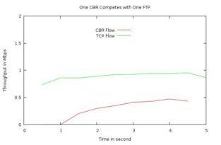
Visualize thr1 and thr2 with gnuplot :

$ gnuplot
gnuplot> set title “One CBR Competes with One FTP”
gnuplot> set xlabel “Time in second”
gnuplot> set ylabel “Throughput in Mbps”
gnuplot> set key 3,1.8
gnuplot> set label “Yield Point” at 0.003,260
gnuplot> set arrow from 0.002,250 to 0.003,280
gnuplot> set xr[0:5]
gnuplot> set yr[0:2]
gnuplot> plot “thr1″ using 1:2 title ‘CBR Flow’ with lines,\
> “thr2″ using 1:2 title ‘TCP Flow’ with lines

Final Result :

this post is taken and modified from http://people.duke.edu/~hpgavin/gnuplot.html and http://alkautsarpens.wordpress.com